2020-04-17
This blog post was originally published as a Towards Data Science article here.
In this blog post, I am going to investigate the serial (aka temporal) dependence phenomenon in random binary sequences.
Random binary sequences are sequences of zeros and ones generated by random processes. Primary outputs generated by most random number generators are binary. Binary sequences often encode the occurrence of random events:
In many of those situations, it is necessary to ensure that the tracked events occur independently of each other. For example, the occurrence of an incident in a production system should not make the system more incident prone. For that, we need to take a close look at the dependence structure of the binary sequence under consideration.
In this blog post, I am going to develop and test a scoring method for quantifying the dependence strength in random binary sequences. The Meixner Dependency Score is easy to implement and is based on the orthogonal polynomials associated with Geometric distribution.
After reading through this blog post, you will know:
Given a sequence of random variables X = (X_0, X_1, ..., X_n) taking values in the set \{0, 1\} and a probability p\in(0,1), I would like to investigate the serial dependencies between the elements of X. This investigation should be based on a sample x drawn from X, i.e. a finite sequence of zeros and ones (x_0, x_1,.., x_n). This is a very difficult and deep problem, and in this blog post I am going to focus on collecting evidence to support or reject the following two basic hypotheses:
If we assume that the elements of x are independent samples from a fixed Bernoulli random variable X_0, then we can estimate the probability p by calculating the average of x_0, x_1, ..., x_n. This is because the expectation of X_0 is \mathbb E X_0 = p.
To set an appropriate context for the serial dependence detection problem, let me remark that random binary sequences x are often associated with discreet observations of a system with two states. We say that “an event” occurred at time i, if x_i = 1.
How can we check whether our events occur independently of each other and gather evidence that there is no serial dependence between the event times?
We often tend to see serial dependence in situations where there is none. Typical examples are the “winning or lucky streaks” experienced by gamblers in casinos.
To rigorously investigate the question of serial dependence in the sequence X based on the observation x, we can look at the distribution of waiting times between the events. For example the sequence
[0, 1, 1, 0, 0, 1, 0, 0]yields the following sequence of waiting times
[1, 3].Note that the waiting time calculation discards the initial and trailing zeros in the event sequence x.
To formally define the waiting time sequence y=(y_1,\ldots,y_m) based on x, consider the sequence of indices I=(i_1,\ldots,i_{m+1}), such that for each i\in I we have x_i=1. We set
y_j = i_{j+1} - i_{j},\text{ for } j = 1,\ldots,m.
For an i.i.d. sequence of Bernoulli random variables, the sequence of waiting times consists of i.i.d. random variables with the geometric distribution. Let’s have a closer look at its properties.
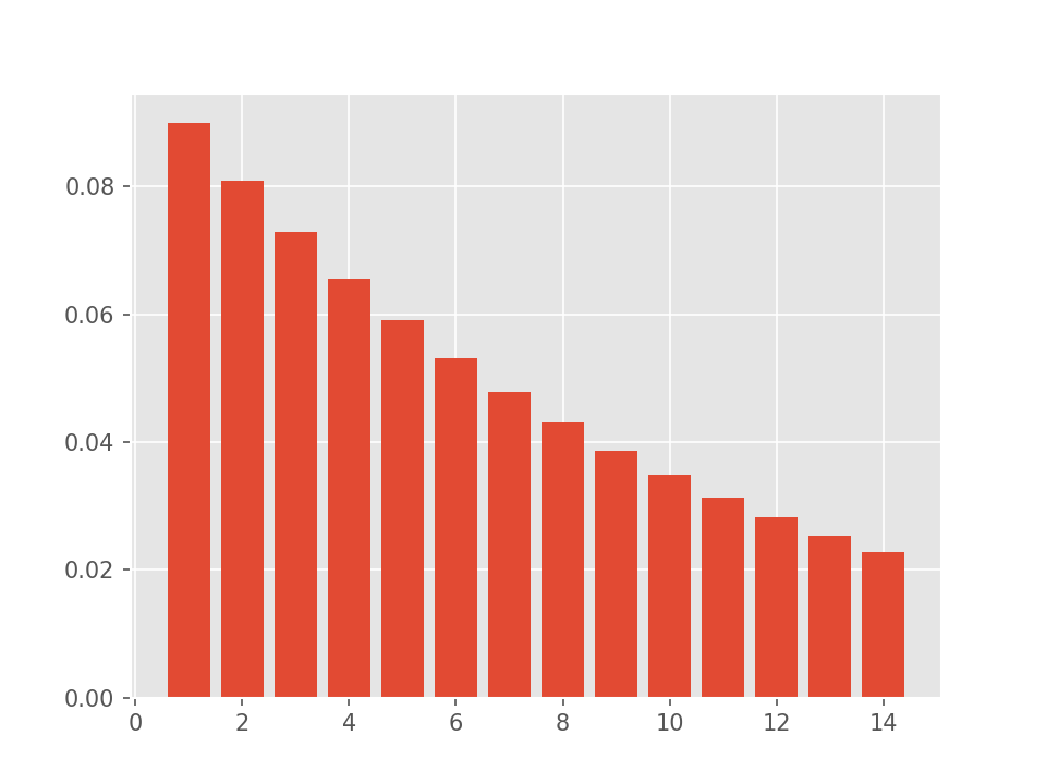
The probability mass function (PMF) of the geometric distribution with parameter p is given by
w(k) = \mathbb P(Z = k) = (1-p)^{k-1} p,\ k=1,2,...
The PMF of the geometric distribution with the parameter p=0.1 looks as follows.
One way of test whether a waiting times sequence follows the geometric distribution is to look at the orthogonal polynomials generated by that distribution.
A family of orthogonal polynomials is intimately tied to every probability distribution \mu on \mathbb R. For any such distribution, we can define a scalar product between (square-integrable) real-valued functions f, g as
\langle f,g \rangle = \int f(y) g(y) \mu(dy) = \mathbb E f(Y)g(Y),
where Y is a random variable with distribution \mu. For a geometric distribution, the above scalar product takes the form
\langle f,g \rangle = \sum_{k\geq 1} f(k) g(k)\, p (1-p)^{k-1}.
We say that the functions f and g are orthogonal (with respect to \mu) if and only if
\langle f,g \rangle = 0.
Finally, a sequence of polynomials (q_i)_{i\geq 0} is called orthogonal, if and only if \langle q_k, q_i \rangle = 0 for all k \neq i, and each q_i has degree i. As a consequence, we have \mathbb E q_i (Y) = 0 for i>0. This is the tool I am going to use to check whether a given Y follows a geometric distribution.
The family of orthogonal polynomials M = (M_i(y))_{i\geq 0} corresponding to the geometric distribution is a special case of the Meixner family derived from the negative binomial distribution (a generalization of the geometric distribution). The members of the Meixner family satisfy the following handy recursive relation:
M_{i+1}(y) = \frac{(1-p)(2i+1) + p(i-y+1)}{(i+1)\sqrt{1-p}} M_i(y) - \frac{i}{i+1} M_{i-1}(y),
with M_1(y) = 1 and M_{-1}(y) = 0. This relation is used to calculate the sequence M. Also, note that M_k depends on the value of the parameter p.
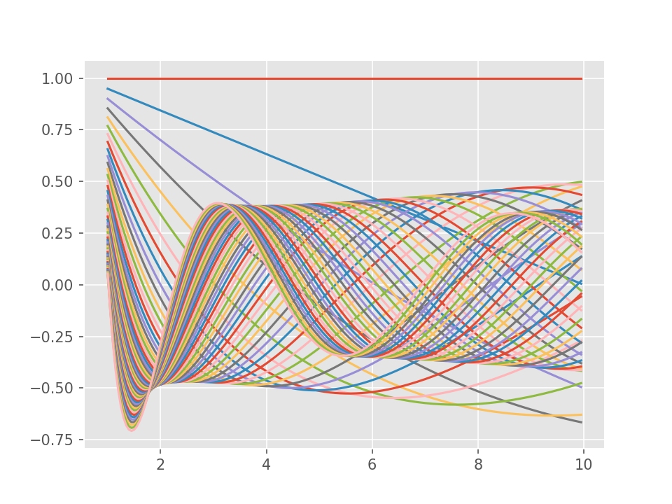
In the companion python source code 1,
the function meixner_poly_eval is used to evaluate Meixner
polynomials up to a given degree on a given set of points. I used this
function to plot the graphs of these polynomials up to degree 50.
As mentioned above, for every polynomial M_k(y) in M the equation
\mathbb E M_k(Y) = 0
holds, if and only if Y\in \text{Geom}(p) and k>0.
This relation can be used to test whether a given sample of waiting times belongs to the geometric distribution with parameter p. We are going to estimate the expectations \mathbb E M_k(Y) and use the estimates as scores: Values close to zero can be interpreted as evidence speaking for geometric distribution with parameter p. If the values are far from zero, this is a sign that we need to revisit our assumptions and possibly discard the i.i.d. hypothesis about the original event sequence. Note that significant deviations from zero can also occur if the events are independent but the true probability \tilde p differs significantly the putative p. This can easily be tested as described earlier.
In order to arrive at a single number (a score) that quantifies the degree of serial dependence in the sense developed above, we will define the Meixner dependency score (MDS) as a mean of expectation estimates for the first k Meixner polynomials evaluated at a sample of waiting times y = (y_1,..,y_m):
D^k_{\text{meixner}}(y) = \frac{1}{k} \sum_{i=1}^{k} |\bar{M}_i(y)|.
The idea of using orthogonal polynomials to test the dependence structure assumptions in binary sequences has its roots in the method of moments inference and was developed in the financial literature to backtest Value-at-Risk models. In this blog post I adapt the approach outlined in Candelon et al. See the References section below.
To find out whether the procedure devised above has a chance to work in practice, I am going to test it using synthetically generated data. This type of a testing procedure is commonly known as Monte-Carlo (MC) study. It doesn’t replace tests with real-world data, but it can help evaluate a statistical method in a controlled environment.
The experiment we are going to perform consists of the following steps:
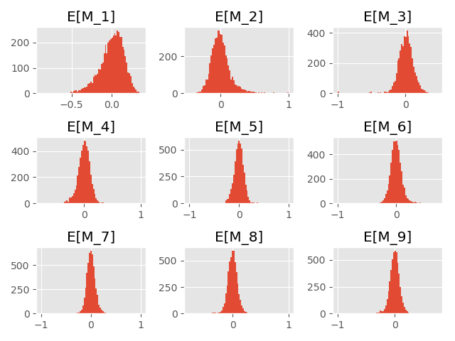
Let’s start with a simple case of simulating an i.i.d. sequence of Bernoulli random variables with success probability p_0 This can be used as a sanity check and to test whether our implementation of the procedure is correct.
For the following experiment we set p_0 = 0.05 and simulate 5000 samples from X = (X_1,.., X_{1000}).
For a model with a simple form of serial dependence, we select the probabilities 0 < p_1 < p_0 < p_2 < 1 and set the distributions of random variables in the sequence X = (X_0, X_1, X_2, ...) as follows. Let X_0 be Bernoulli with success probability p_0. The distributions of X_i for i>0 are conditional on X_{i-1}:
\begin{aligned} \mathbb P(X_i = 1 | X_{i-1} = 0) &= p_1, \\ \mathbb P(X_i = 1 | X_{i-1} = 1) &= p_2. \end{aligned}
In order to compare this model with an i.i.d. Bernoulli model with the success probability p_0, we need to set p_1 and p_2 such that the unconditional distributions of X_i are \text{Ber}(p_0).
In other words, for a given 0 < p_1 < p_0 < 1, we are looking for a p_2\in (0, 1), such that the random binary sequence defined above satisfies P(X_i = 1) = p_0. This binary sequence can be represented as a simple Markov chain with the state space \{0, 1\}, the transition probability matrix P given by
\left(\begin{matrix} 1-p_1 & p_1 \\ 1-p_2 & p_2 \end{matrix}\right),
and the initial distribution \lambda = (1-p_0, p_0). The marginal distribution of X_i is given by \lambda P^i. This basic result can be found in any book about Markov Chains (see the References section below). The task of finding a p_2 such that \mathbb P (X_{i} = 1) is as close to p_0 as possible, can be easily solved with an off-the-shelf optimization algorithm such as BFGS.
For example, the above procedure quickly yields p_2 = 0.62 for p_1 = 0.02 and p_0 = 0.05.
Let’s test the dependency scoring algorithm for the following values p_1 and p_2. An MC evaluation of the Meixner polynomials leads to the following Meixner dependency scores:
| p1 | p2 | MDS |
|---|---|---|
| 0.5 | 0.5 | 0.083 |
| 0.4 | 0.24 | 0.194 |
| 0.3 | 0.43 | 0.382 |
| 0.2 | 0.62 | 0.583 |
Again, 5000 simulations of samples of length 1000 yield the following histograms for the expectation estimates.
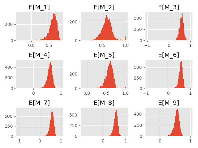
As we can see, the histograms are shifted slightly to the left.
All the results and plots presented in this blog post have been generated using the following Python script: meixner.py
In this blog post, we learned about the concept of serial dependence in binary sequences. We implemented a serial dependence detection method, the Meixner Dependency Score, based on the Meixner orthogonal polynomials and tested its performance using a simple Markov chain model.
An important financial use case for dependency testing is the analysis of the Value-at-Risk exceedance event sequence generated by a market risk model. Market Risk models are widely used in the banking industry for regulatory capital requirement calculations and in the asset management industry for portfolio construction and risk management.
The Value-At-Risk (Var) is a quantile of the loss distribution for a financial asset price over a fixed time horizon. For example, an investor holding a long position in gold may be interested in the 95% VaR over a one-day time horizon for the gold price in USD. For a well-calibrated VaR model, the extreme losses on 5% of the business days observed over an investment period will exceed the 95% VaR score. The VaR exceedance events must not only occur with the expected frequency but must also be independent of each other. Proper calibration of the market risk model that brings the dependency of the exceedance events to a low level is typically much more difficult than simple calibration of the exceedance frequency. But this is especially important in the times of financial distress, because underestimating the risk leads inevitably to underhedging, and, possibly, to more severe losses.
Many thanks to Sarah Khatry for reading drafts of this blog post and contributing countless improvement ideas and corrections.