In this post I introduce a class of discrete stochastic volatility models using a nice notation and go over some special cases including GARCH and ARCH models. I show how to simulate these processes and how parameter estimation performs. The Python code I wrote for these experiments is referenced at the end of the post.

Discrete stochastic volatility models

If you are not that familiar with the probability theory, do yourself a favor and just read over the mathematical intricacies, or maybe skip right ahead to the “special cases” section and pick the details from here only of they seem relevant to you.

\global\def\Xpred#1{(X_s)_{s\lt #1}}

Let \left( \Omega, \mathcal A, \mathcal F, P \right) be a stochastic basis with a complete \sigma-algebra \mathcal A of measurable subsets of \Omega, a probability measure P, and a filtration \mathcal F = (\mathcal F_t)_{t=0, 1, \ldots}.

• Thus, the time instances are indexed using non-negative integers 0, 1, \ldots.

• To get the first t elements of a sequence X = (X_0, X_1, \ldots), I use the notation \Xpred{t} = (X_0,\ldots,X_{t-1}).

  A discrete stochastic volatility (DSV) model X = (X_0, X_1, \ldots) is a real-valued stochastic process (a sequence of random variables) satisfying the following equations:

\begin{aligned} X_t &= \mu_t + \sigma_t Z_t \\ \mu_t &= \phi_0 + \sum_{i=1}^{p} \phi_i f_i (\Xpred{t}) \\ \sigma_t^2 &= \gamma_0 + \sum_{i=1}^q \gamma_i g_i(\Xpred{t}) + \sum_{i=1}^r \lambda_i h_i((\sigma_s^2)_{s\lt t}). \end{aligned}

Ingredients:

• Z is a noise process adapted to \mathcal F, such that Z_t are i.i.d. copies of a random variable with density \eta_Z.
• \phi_i are real numbers and, to avoid trouble, I assume that \gamma_i, \lambda_i \geq 0 and that g_i, h_i are non-negative valued.
• f_i, g_i, and h_i are deterministic functions of the process.
• The process \mu is often called the drift, whereas \sigma is called the volatility of X. Because \sigma is a stochastic process, the process X as defined above belongs to a large family of stochastic volatility models.
• For a noise process Z such that the mean and the variance of every Z_t exist, we have \mathbb E [X_t | \mathcal F_{t-1}] = \mu_t and \operatorname{Var} [X_t | \mathcal F_{t-1}] = \sigma^2_t.

Special cases

To formulate the specializations of the general DSV model the following notation comes in handy.

The backward shift operator B^j, for j\geq 0, produces a delayed version of its argument process, i.e. B^j (X)_t = X_{t-j}, if t-j \geq 0, and B^j (X)_t = 0, if t-j \lt 0. For example

B^1(X) = B(X) = (0, X_1, X_2, \ldots).

For convenience, I set B^1 = B and B^j_t (X) = B^j(X)_t = X_{t-j}.

For all the special cases in the list below, I assume that the functions f_i, g_i, and h_i pick a single element from the history of the argument process, i.e. f_i = h_i = B^i_t, and g_i(\Xpred{t}) = B^j_t(X^2).

GARCH process definitions found in textbooks additionally set \mu\equiv 0.

The GARCH(1, 1) processes are quite popular, so let’s stat the dynamics explicitly:

\begin{aligned} X_t &= \sigma_t Z_t \\ \sigma_t^2 &= \gamma_0 + \gamma_1 B_t(X^2) + \lambda_1 B_t(\sigma^2). \end{aligned}

In an ARCH process, the volatility has the simplified form with \lambda_i = 0 for all i, and \mu \equiv 0.

\begin{aligned} X_t &= \sigma_t Z_t \\ \sigma_t^2 &= \gamma_0 + \sum_{i=1}^q \gamma_i B^i_t(X^2). \end{aligned}

An ARCH(1) process additionally satisfies \gamma_i = 0 for all i \geq 2:

\begin{aligned} X_t &= \sigma_t Z_t \\ \sigma_t^2 &= \gamma_0 + \gamma_1 B_t(X^2). \end{aligned}

Simulation

Discrete stochastic volatility models are typically used to model the log-returns of an observed time-series. Therefore in order to simulate a path of the original time-series we need to simulate its log-returns and calculate Y = Y_0 \prod_{s=0}^t \exp(X_s).

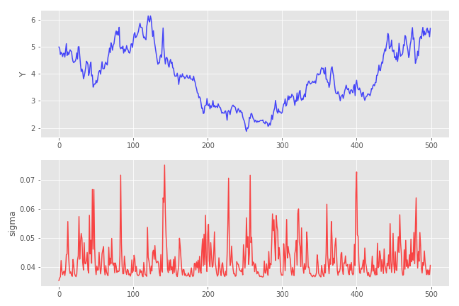
A sample path of a GARCH(1,1) process driven by the Gaussian noise with parameters (\gamma_0, \gamma_1, \lambda_1) = (0.001, 0.2, 0.25):

Note that the \sigma process for t>0 cannot go below the level of \sqrt{\gamma_0 (1 + \lambda_1)} \approx 0.0353

Maximum-likelihood estimation

Maximum-likelihood (ML) parameter estimation is the method of choice for all the discussed models since the transition density, i.e. the density of X_t given the past information \mathcal F_{t-1} is known explicitly. Log-likelihood function of the process sample path x is thus given by

\ln L(\theta; x) = \sum_{s=1}^t \ln \eta_Z \left( \frac{x_t - \mu_t(\theta)}{\sigma_t(\theta)} \right) - \ln \sigma_t(\theta),

where \theta = (\phi_i, \gamma_i, \lambda_i), and \eta_Z is the density of Z. Minimizing the above log-likelihood function yields the maximum-likelihood estimate \hat\theta for \theta:

\hat\theta(x) = \operatorname{argmin}_{\theta} \ln L(\theta; x).

Monte-Carlo study

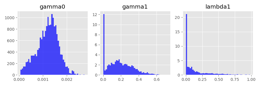
In order to test the ML parameter estimation procedure, I perform the following Monte-Carlo experiment.

• Simulate 2500 independent GARCH(1,1) process paths of length 5000 with parameters (0.001, 0.2, 0.25). I used the Gaussian noise, i.e. Z_t \sim\mathcal N(0,1).
• Feed each of these paths to the ML estimator and get the estimated parameter vectors (\hat\theta_i)_{i=1,\ldots, 2500}.
  • The search ranges for parameters in this optimization procedure are restricted to [1e-8, 1].
• Compare original \theta with the estimated \hat\theta_i.
• Simulate GARCH(1,1) with parameter vectors \hat\theta_i, calculate means and standard deviations, and compare these to the “true” mean and standard deviation (which are 5.098 and 1.084, respectively).

As expected, the estimator \hat\theta is very inaccurate and, in most cases, doesn’t even come close to the true vector \theta. In particular, the estimated \gamma_1 and \lambda_1 are often set to zero (see the histograms below).

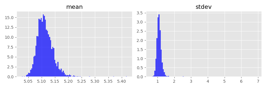
On the other hand, the process means and standard deviations coming from the estimated \hat\theta are much more accurate. This is a good thing, because we usually care more about recovering the characteristics of the unknown data generating process and not so much about the true parameter values of the model.

Crazy idea: The Cauchy driving noise

The noise process Z doesn’t have to be normalized to mean 0 and variance 1. In fact, we just need to make sure that the distribution of the random variable Z_t admits a density. If this is the case, both, process simulation and ML estimation work as described.

So how about replacing the Gaussian noise with a noise sampled from the Cauchy distribution? In many probability theory books, the Cauchy distribution is used a counterexample, because it has many “pathological” properties. For example, it has no mean and, consequently, no variance. (“No mean” means that the integral used to define the first moment diverges, i.e. has no finite value.)

This is the theory which I learned few years ago. What I didn’t know is how erratic samples from a Cauchy distribution look like. Just take a look at a sample path of the GARCH(1,1) process with the parameter vector (\gamma_0, \gamma_1, \lambda_1) = (0.0001, 0.001, 0.01):

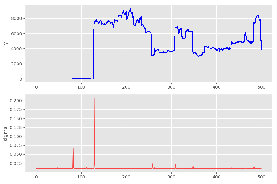
If you play around with the path generating function long enough, you may even generate a floating point overflow exception. The Python function I used to generate histograms shown above fails because of that. To see what is going on under the hood, let’s generate some histograms using samples from the Cauchy distribution:

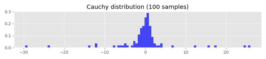
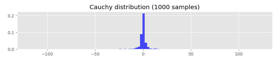
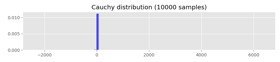
The Cauchy distribution has the quantile function

Q(p) = \tan (\pi (p-0.5)).

Evaluating Q(1-p) for p=0.01, 0.001, 0.0001 gives

Q(0.99) ~= 31.82
Q(0.999) ~= 318.31
Q(0.9999) ~= 3183.10

This means that, for example, with probability of 0.0001 the sampled values are greater than 3183.10. For comparison, let’s calculate the corresponding quantiles of the standard normal distribution:

> from scipy.stats import norm
> print(norm.ppf(0.99))
2.32
> print(norm.ppf(0.999))
3.09
> print(norm.ppf(0.9999))
3.71

References and Links

• The python module used to generate the plots shown in this post is here: garch.py.
• https://en.wikipedia.org/wiki/Cauchy_distribution
• McNeil, Alexander J., Rüdiger Frey, and Paul Embrechts. Quantitative risk management. Princeton university press, 2015. (This book contains one short chapter nicely summarizing univariate time-series models.)